Intuitive Physics Net
Motivation
Early on in our development, human beings cultivate an intuition as to how objects in the physical world should behave. We understand that if we throw a ball into the air, it will travel in a roughly parabolic trajectory before hitting the ground. We know that if we roll that same ball across the surface of a table, it will eventually come to a stop. Moreover, we understand if we throw it towards a wall, it will bounce back. We know these things without explicitly being given the equations that describe the objects’ motion. Our physical intuition is developed over time by interacting with and observing the world.
The purpose of my project is to build a network that can learn the rules of how objects move in space in the same manner that humans learn those rules - via observation and without explicit definition of concepts like momentum, force, or friction.
To train the network, I asked it to perform a task that most people would find fairly simple. Given two frames of a video in which some number of objects are moving, predict the positions of those objects in the following frame.
Let’s say we have a recording of circles moving within a closed space and I showed you two sequential frames:
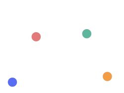
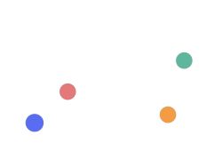
You’re likely able to roughly intuit the vectors describing the motion of the circles.
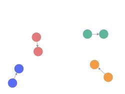
Having intuited the circles’ motion vectors, you are then able to guess at the position of the circles in the next frame.
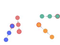
During training, the network is fed two frames and asked to guess at what the third frame should look like.
Generating Data
To start, data will have to be generated. This was done by creating environments using the matter.js physics engine.
<html>
    <head>
    </head>
    <body>
        <script src="matter.js"></script>
        <script src="index.js"></script>
    </body>
</html>
// index.js
// module aliases
var Engine = Matter.Engine,
Render = Matter.Render,
World = Matter.World,
Body = Matter.Body,
Bodies = Matter.Bodies;
var engine = Engine.create();
var render = Render.create({
element: document.body,
engine: engine,
options:{
height: 600,
width: 600,
background: '#222',
showVelocity: false,
wireframes: false
}
});
// create boundaries of environment
var ground = Bodies.rectangle(0, 590, 1200, 20, { isStatic: true });
var ceiling = Bodies.rectangle(400, 10, 810, 20, { isStatic: true });
var leftWall = Bodies.rectangle(10, 120, 20, 1000, { isStatic: true });
var rightWall = Bodies.rectangle(590, 120, 20, 1000, { isStatic: true });
function generateCircles(){
var numCircles = Math.floor(Math.random() * 5) + 1;
var circles = [];
for (i = 0; i < numCircles; i++){
// randomly generate the x and y coordinates of each of the circles
var x_coord = Math.floor(Math.random() * 700);
var y_coord = Math.floor(Math.random() * 500);
//randomly generate the color of the inside of the circle as well
// as its boundary
var fillColor = '#'+Math.floor(Math.random()*16777215).toString(16);
var strokeColor = '#'+Math.floor(Math.random()*16777215).toString(16);
// each circle has a radius of 30. The 'restitution' attribute refers to
// the elasticity of the collisions between circles. Setting it to '1.0'
// configures the circles to have the same kinetic energy before and
// after collisions.
// Setting inertia to infinity ensures that the circles have no angular
// velocity (otherwise the circles slow down).
var ball = Bodies.circle(x_coord, y_coord, 30, {
density: 0.04,
friction: 0.00,
frictionAir: 0.0000,
restitution: 1.0,
inertia: Infinity,
render: {
fillStyle: fillColor,
strokeStyle: strokeColor,
lineWidth: 2
}
});
// Set the velocity of the circle to a random value
x_sign = [-1, 1][Math.floor(Math.random() * 2)];
y_sign = [-1, 1][Math.floor(Math.random() * 2)];
x_velocity = Math.floor(Math.random() * 16) * x_sign;
y_velocity = Math.floor(Math.random() * 16) * y_sign;
Body.setVelocity(ball, { x: x_velocity, y: y_velocity })
circles.push(ball)
}
World.add(engine.world, circles);
}
generateCircles();
// add all of the bodies to the world
World.add(engine.world, [ground, ceiling, leftWall, rightWall]);
engine.world.gravity.y = 0;
Engine.run(engine);
Render.run(render);
Of course, we still need to record the canvas in which the matter.js environment is rendered. This code is a modification of a WebRTC example that can be found here.
let mediaRecorder;
let recordedBlobs;

const canvas = document.querySelector('canvas');

// returns a MediaStream object which has a recording of the canvas
const stream = canvas.captureStream();
console.log('Started stream capture from canvas element: ', stream);

function handleDataAvailable(event) {
  if (event.data && event.data.size > 0) {
    recordedBlobs.push(event.data);
  }
}

function startRecording() {
  let options = { mimeType: 'video/webm' };
  recordedBlobs = [];

  mediaRecorder = new MediaRecorder(stream, options);

  console.log('Created MediaRecorder', mediaRecorder, 'with options', options);
  mediaRecorder.ondataavailable = handleDataAvailable;
  mediaRecorder.start(100);
  console.log('MediaRecorder started', mediaRecorder);
}

function stopRecording() {
  mediaRecorder.stop();
  console.log('Recorded Blobs: ', recordedBlobs);
}

function download() {
    const blob = new Blob(recordedBlobs, {type: 'video/webm'});
    const url = window.URL.createObjectURL(blob);
    const a = document.createElement('a');
    a.style.display = 'none';
    a.href = url;
    a.download = 'train_vid_' + localStorage.getItem("sampleCount") + '.webm';
    document.body.appendChild(a);
    a.click();
    setTimeout(() => {
        document.body.removeChild(a);
        window.URL.revokeObjectURL(url);
    }, 100);
}

function stopAndDownload() {
    if (!localStorage.getItem("sampleCount")){
        localStorage.setItem("sampleCount", '000');
        console.log(localStorage.getItem("sampleCount"));
    } else {
        previous_count = parseInt(localStorage.getItem("sampleCount"));
        localStorage.setItem("sampleCount", (previous_count + 1).toString().padStart(3, '0'));
        console.log(localStorage.getItem("sampleCount"));
    }

    stopRecording();
    download();
    setTimeout(refreshPage, 3000);
}

function refreshPage() {
    window.location.reload();
}

startRecording();
setTimeout(stopAndDownload, 6000);
localStorage.clear() can be used to reset sampleCount if you need to generate multiple datasets.
The next steps are to extract the frames from the webm files we’ve recorded and then to separate those files into features and labels. We’ll use ffmpeg to do so.
#!/bin/bash

# extract_frames.sh
# iterates through webmfiles and extracts frames from each
# frames are placed in the training_set or test_set directory
# the frames are named like so:
# "train_img_[webmfile number]_[frame number]"/"test_img_[webmfile number]_[frame number]"

# `sort -n -t _ -k 3` sorts the files numerically using the third part of the
# file name, where the separator is the underscore. This works because the
# webmfiles are named like so: train_vid_[video number]/test_vid_[video number]

for filename in $(ls webmfiles/training/*.webm | sort -n -t _ -k 3); do
  num=$(echo "$filename" | grep -o '[0-9]\+')

  img_file="./training_set/train_img_${num}_%03d.jpeg"

  ffmpeg -i $filename -r 21 -s 28x28 -frames:v 105 -f image2 $img_file
done

for filename in $(ls webmfiles/test/*.webm | sort -n -t _ -k 3); do
  num=$(echo "$filename" | grep -o '[0-9]\+')

  img_file="./test_set/test_img_${num}_%03d.jpeg"

  ffmpeg -i $filename -r 21 -s 28x28 -frames:v 105 -f image2 $img_file
done
#!/bin/bash
# split_training.sh
# iterates through files in the training and test sets and separates the files in each into
# features and labels (i.e. target values)
for filename in $(find ./training_set/ -maxdepth 2 -name "*.jpeg"); do
# nums looks like "[video number] [image number]"
nums=$(echo $filename | ggrep -oP '[0-9]+')
vid_num=$(echo $nums | ggrep -oP '[0-9]+\s')
zero_pad_img_num=$(echo $nums | ggrep -oP '\s[0-9]+')
# get the non-zero-padded image number so the modulo operator
# can be used on it
img_num=$(echo $zero_pad_img_num | sed 's/^0*//')
file_basename=$(basename $filename)
if (($img_num % 3 == 0)); then
mv "./training_set/$file_basename" "./training_set/labels/$file_basename"
else
mv "./training_set/$file_basename" "./training_set/features/$file_basename"
fi
done
for filename in $(find ./test_set/ -maxdepth 2 -name "*.jpeg"); do
nums=$(echo $filename | ggrep -oP '[0-9]+')
vid_num=$(echo $nums | ggrep -oP '[0-9]+\s')
zero_pad_img_num=$(echo $nums | ggrep -oP '\s[0-9]+')
img_num=$(echo $zero_pad_img_num | sed 's/^0*//')
file_basename=$(basename $filename)
if (($img_num % 3 == 0)); then
mv "./test_set/$file_basename" "./test_set/labels/$file_basename"
else
mv "./test_set/$file_basename" "./test_set/features/$file_basename"
fi
doneConvolutional Autoencoder
An autoencoder is a kind of neural network that reduces its input to a lower-dimensional coding (i.e. a simpler representation) and outputs a reconstruction of the input using that coding.
As an example, let’s take something complex, like a cat, and reduce it to its most important characteristics.
Fluffy
- long tail
- pointy ears
- whiskers
- four legs
- has fur
- enjoys catching mice
- has orange stripes
- sits on your keyboard when you’re trying to work
- scratches your face in the morning for no damn reason
- poops around, but not in, the litter box
- will not play with expensive toy you purchased, but will gnaw on your shoes
These are the most salient features of Fluffy, and if Fluffy were to somehow pass away doing something stupid like, say, running headfirst into a window whilst attempting to chase a bird that’s outside, we would very easily be able to clone him (but, why would you?).
In FlowNet: Learning Optical Flow with Convolutional Networks (also see this demo), pairs of adjacent frames are stacked and then passed as input to a series of convolutional layers. The output of those convolutional layers is then passed through a series of upsampling (or deconvolutional) layers which, in turn, output an image.
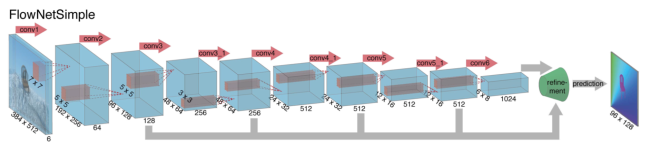
Flownet returns an optical flow field i.e. an image that highlights the objects whose position changes between the first and second frames. My network is an implementation of this architecture in which the output is, instead, the next frame in the sequence. It’s heavily inspired by Felix Mohr’s implementation of a variational autoencoder.
Here is the network in its entirety.
import tensorflow as tf
import cv2
import os
import numpy as np
import matplotlib.pyplot as plt

# Data Loading and Transforming

features_path = "./training_set/features/"
labels_path = "./training_set/labels/"

test_features_path = "./test_set/features"
test_labels_path = "./test_set/labels"

def load_data(img_dir):
    all_imgs = []
    for img in sorted(os.listdir(img_dir)):
        if img.endswith(".jpeg"):
            image = cv2.imread(os.path.join(img_dir, img))
            all_imgs.append(image)
    return np.array(all_imgs)

def concat_frames(samples):
    num_samples = samples.shape[0]
    paired_samples = np.array(np.split(samples, num_samples / 2))

    concatenated_frames = []

    for pair in paired_samples:
        concatenated_frames.append(np.concatenate((pair[0], pair[1]), axis=2))

    return np.array(concatenated_frames)

def scale_pixel_values(samples):
    return samples / 255

def get_next_batch(num_samples, batch_size):
    # shuffle training set
    indices = np.random.randint(0, num_samples, batch_size)
    # take the red channel from RGB images
    return paired_frames[indices,:,:,:], label_imgs[indices,:,:,:]

# Training Data
# frames are 28 x 28 x 3
feature_imgs = load_data(features_path)
label_imgs = load_data(labels_path)

# scale image values to [0, 1]
feature_imgs = scale_pixel_values(feature_imgs)
label_imgs = scale_pixel_values(label_imgs)

# stack feature images
# when frames are stacked, samples are 28 x 28 x 6
paired_frames = concat_frames(feature_imgs)


# Test Data
test_feature_imgs = load_data(test_features_path)
test_label_imgs = load_data(test_labels_path)

test_feature_imgs = scale_pixel_values(test_feature_imgs)
test_label_imgs = scale_pixel_values(test_label_imgs)

test_paired_frames = concat_frames(test_feature_imgs)

# Model
tf.reset_default_graph()

batch_size = 64

X = tf.placeholder(dtype=tf.float32, shape=[None, 28, 28, 6], name='X')
Y = tf.placeholder(dtype=tf.float32, shape=[None, 28, 28, 3], name='Y')
Y_flat = tf.reshape(Y, shape=[-1, 28 * 28 * 3])
keep_probability = tf.placeholder(dtype=tf.float32, shape=(), name='keep_probability')

def encoder(X, keep_probability):
    with tf.variable_scope("encoder", reuse=None):
        X_reshaped = tf.reshape(X, shape=[-1, 28, 28, 6])
        x = tf.layers.conv2d(X_reshaped, filters=64, kernel_size=4, strides=2, padding='same', activation=tf.nn.relu)
        x = tf.nn.dropout(x, keep_probability)
        x = tf.layers.conv2d(x, filters=64, kernel_size=4, strides=2, padding='same', activation=tf.nn.relu)
        x = tf.nn.dropout(x, keep_probability)
        x = tf.layers.conv2d(x, filters=64, kernel_size=4, strides=1, padding='same', activation=tf.nn.relu)
        x = tf.nn.dropout(x, keep_probability)
        x = tf.contrib.layers.flatten(x)
        return tf.layers.dense(x, units=64)


def decoder(coding, keep_probability):
    with tf.variable_scope("decoder", reuse=None):
        x = tf.layers.dense(coding, units=7*7*3, activation=tf.nn.relu)
        x = tf.reshape(x, [-1, 7, 7, 3])
        x = tf.layers.conv2d_transpose(x, filters=64, kernel_size=4, strides=2, padding='same', activation=tf.nn.relu)
        x = tf.nn.dropout(x, keep_probability)
        x = tf.layers.conv2d_transpose(x, filters=64, kernel_size=4, strides=1, padding='same', activation=tf.nn.relu)
        x = tf.nn.dropout(x, keep_probability)
        x = tf.layers.conv2d_transpose(x, filters=64, kernel_size=4, strides=1, padding='same', activation=tf.nn.relu)
        x = tf.contrib.layers.flatten(x)
        x = tf.layers.dense(x, units=28*28*3, activation=tf.nn.sigmoid)
        img = tf.reshape(x, shape=[-1, 28, 28, 3])
        return img


encoding = encoder(X, keep_probability)
decoded = decoder(encoding, keep_probability)

decoded_flat = tf.reshape(decoded, [-1, 28*28*3])
img_loss = tf.reduce_sum(tf.squared_difference(decoded_flat, Y_flat), 1)
loss = tf.reduce_mean(img_loss)
training_op = tf.train.AdamOptimizer(0.0001).minimize(loss)


init = tf.global_variables_initializer()

with tf.Session() as sess:
    init.run()
    for epoch in range(30000):
        x_batch, y_batch = get_next_batch(3640, batch_size)
        sess.run(training_op, feed_dict = {X: x_batch, Y: y_batch, keep_probability: 0.80})

        if not epoch % 200:
            ls, d = sess.run([loss, decoded], feed_dict = {X: x_batch, Y: y_batch, keep_probability: 1.0})
            plt.subplot(1,2,1)
            plt.imshow(np.reshape(y_batch[0], [28, 28, 3]))
            plt.subplot(1,2,2)
            plt.imshow(d[0])
            plt.show()
            print(epoch, ls)

    # Evaluation
    print("Evaluation")
    x_test = test_paired_frames
    y_test = test_label_imgs
    ls, d = sess.run([loss, decoded], feed_dict = {X: x_test, Y: y_test, keep_probability: 1.0})
    plt.subplot(1,2,1)
    plt.imshow(np.reshape(y_test[0], [28, 28, 3]))
    plt.subplot(1,2,2)
    plt.imshow(d[0])
    plt.show()
    print(ls)

# save target frames
count = 0
for i, concatenated in enumerate(test_paired_frames[0:140, :, :, : ]):
    split = np.split(concatenated, 2, axis=2)

    frame1 = split[0] * 255
    frame2 = split[1] * 255
    frame3 = test_label_imgs[i] * 255

    frame1_fname = "actual_" + str(count).zfill(3) + ".jpeg"
    frame2_fname = "actual_" + str(count + 1).zfill(3) + ".jpeg"
    frame3_fname = "actual_" + str(count + 2).zfill(3) + ".jpeg"

    path = "./vid_frames_actual/"
    cv2.imwrite(os.path.join(path, frame1_fname), frame1)
    cv2.imwrite(os.path.join(path, frame2_fname), frame2)
    cv2.imwrite(os.path.join(path, frame3_fname), frame3)

    count += 3

# save predicted frames
count = 0
for i, concatenated in enumerate(test_paired_frames[0:140, :, :, : ]):
    split = np.split(concatenated, 2, axis=2)

    frame1 = split[0] * 255
    frame2 = split[1] * 255
    frame3 = d[i] * 255

    frame1_fname = "predicted_" + str(count).zfill(3) + ".jpeg"
    frame2_fname = "predicted_" + str(count + 1).zfill(3) + ".jpeg"
    frame3_fname = "predicted_" + str(count + 2).zfill(3) + ".jpeg"

    path = "./vid_frames_predicted/"
    cv2.imwrite(os.path.join(path, frame1_fname), frame1)
    cv2.imwrite(os.path.join(path, frame2_fname), frame2)
    cv2.imwrite(os.path.join(path, frame3_fname), frame3)

    count += 3
Within the encoder function, we define the network’s convolution layers (for a more in-depth explanation of convolutional neural networks, see this blog post). We specify sixty-four 4x4 kernels at each convolution layer. Sandwiched between the layers are 2 dropout layers to prevent overfitting.
In a standard convolutional autoencoder, the goal is for the network to reconstruct the input image. The convolution layers, in this case, discern the features that are most important for accurately reconstructing the input.
The network above is a variation on that. Instead, the network is trained to output the frame following the input, which is the two proceeding frames stacked along the z-axis. The decoder specifies transpose (i.e. deconvolutional) layers that perform the reconstruction.
On the left is the target animation, i.e. the animation containing the target frames. On the right is the animation containing the frames predicted by the network. You’ll note that the network is less accurate when it comes to returning the correct colors than it is in placing the circles in the correct position.

You can find the code above and training samples on Github.
You can download a more detailed description of my work here.
Reflections on the OpenAI Scholarship
The past three months have been…I can’t quite find a single adjective that would describe the experience accurately.
For 13 weeks, I’ve been able to focus on a topic I find incredibly fascinating. I experienced the joy and excitement that comes with making progress and also the self-doubt and despair that attends failure. It’s been quite the intellectual journey and one I’m glad I didn’t have to take on alone.
I’m extremely thankful to my mentor, Igor Mordatch and our program director Larissa Schiavo. I’m also grateful to have been able to work alongside my fellow scholars, all of whom are brilliant, inspiring, and generous human beings. We’re not quite ready to stop working with each other and we may have some projects lined up that we’ll collaborate on (hint hint).
I know I’ve still a long way to go, but I’m proud of the progress I’ve made. When I started this program, I’d not trained a single neural network. I’d read and written about them, but I had zero hands-on experience. Machine learning is not an easy topic, but now I feel less like I’m trying to scale Mt. Everest and more like I’m climbing up a ladder. Knowing the path forward makes the way shorter.
There were a few things I could have done better. First, I started neglecting things like exercise and regular meditation, both of which are crucial to staying physically and mentally healthy. It’s easy to drop these by the wayside in pursuit of other goals. It’s important to remember that, without them, other goals are so much more difficult to achieve.
Secondly, I waited too long to start writing code, which meant I felt like I was scrambling to pick up enough skill in TensorFlow to build something interesting. Spending half of your day coding and half studying (or whatever proportion you prefer) is a good way to try to prevent this. Even so, it’s hard to shake the idea that if you just read a little more, your code would be better. Of course, it would. But if you write more code…your code will be better. Having said that, I definitely understand the irritation of having only partial knowledge of something, yet trying to build it.
Third, I should have taken weekends off. I didn’t and now I feel super burned out.
As far as the future goes, I have a better idea of what I’d like to do, but things are still a little up in the air. Having said that, I’m going to take a few weeks to rest and get back to Muay Thai.
Photo by Nik MacMillan on Unsplash